Skip to main content
Search
Search This Blog
Data in science, Stats, Coding and Brain Imaging
Thoughts, opinions, code with a zest of brain imaging and open science.
Home
More…
Posts
Latest posts
October 23, 2023
Rewriting history - Git history that is
February 19, 2023
GDPR for research demystified
September 24, 2022
Euler in the brain
May 27, 2022
Neural Oscillations
May 22, 2022
EU scientific data processing and sharing (2/2)
May 21, 2022
EU scientific data processing and sharing (1/2)
April 29, 2021
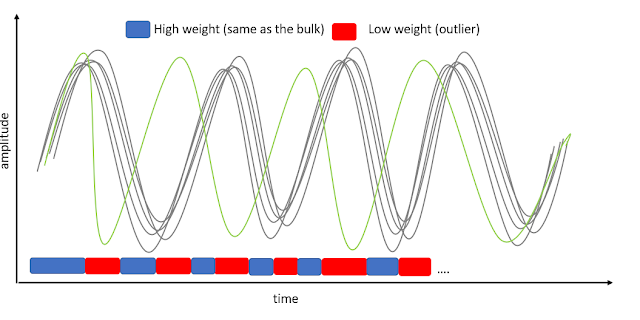
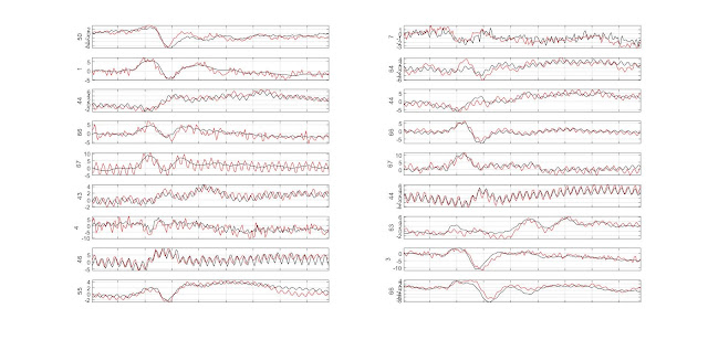
GLM single trial weighting for EEG
January 05, 2021
MEEG single trial metrics
Older Posts