Bootstrapping and multiple comparisons correction in EEG

Re-interpreting BOLD signal activation levels

This blog-post was inspired by the cogneuro subreddit discussing Russ Plodracks' article on neural efficiency: Is “efficiency” a useful concept in cognitive neuroscience? Dev. Cog. Neurosc 2014. I do not discuss here the concept of efficiency (done much better in the article) - instead I discuss some possible analyses that can help interpreting BOLD differences, on the bases of the explanations given by Russ Poldrack in his article.

Quick reminder: what does the BOLD signal reflect?

In a nutshell, we know that the BOLD signal reflects the firing of neural populations such as a strong correlation exists between the BOLD amplitude and local field potentials data (Logothetis, 2001). This means that BOLD is more related to synaptic activity than neural activity (i.e. the interplay of EPSP and IPSP). The BOLD signal increases according to a compressive, non-linear, saturating function of stimulus energy. Indeed, the neural response itself may depend non-linearly on the stimulus energy and the BOLD signal then non-linearly depends on the neural signal (Logothetis and Wandell, 2004).

While a positive BOLD means increased neural activity / increased synaptic activity, a negative BOLD signal seems to reflect neural decrease (Shmuel et al. 2006, Pasley et al., 2007). Current understanding is that synaptic activity related to excitatory (EPSP) and inhibitory (IPSP) potentials leads to observe a positive BOLD response; but a decrease in local neural activity (e.g. related to neighbouring increase of neural activity that locally inhibit neural spiking - see however Devor et al, 2005) leads to a negative BOLD response.

According to Cardoso et al., 2012, the evoked BOLD response is better seen as a linear sum of stimulus induced spiking activity (~50% of the variance in their data) and a trial-related signal (anticipatory? – attention?), not related directly to the local spiking.  Finally, we also know that behind the evoked response, there is the 'resting state' fluctuations, and these two are sub-additive.

Interpreting differences between 2 groups or 2 conditions

A different set of cognitive processes is being performed. 

Poldrack gives as an example a child with Tourette syndrome who, in effect, is in a dual task situation: performing the specified cognitive task + actively attempting to his/her tics. In contrast, a healthy child would not experience this secondary response inhibition demand.There is obviously not much we can do in terms of analysis here - it's all about design. I think that in a case like this one, we can try to elicit inhibition demand in controls to find out if there are overlapping regions with the experimental condition from patients, but that's about it.

In general, it is recommended to control task demand, for instance using an adaptive algorithm to maintain a certain level of performances (when it's possible). I would also add that additional off-scanner questionnaires can be useful - few years ago using such questionnaire we differentiated high vs. low imagers (people how can / can't visualize objects in their mind) who rely on different strategies to rotate objects (e.g. here). It turns out that these different strategies also corresponded with a different level of activation in different regions like the visual and premotor cortex - with the BOLD response following the rotation angles in the pre-motor area, but for high imagers only (paper here). So even in controls, we can have different strategies - it's all about cognition here ...  

A different neural computation is performed to complete the same task. 

The example is that 'in an pseudoword pronunciation task, one group pronounces the stimulus through grapheme-to-phoneme conversion, while a more skilled group pronounces it using analogy to known words. Alternatively, one group represents a stimulus domain using a dense coding scheme, whereas another represents it using sparse coding.' The argument is that 'changes in the nature of neuronal information coding could also result in differences in activation'. Here I would say that fortunately we have a bunch of fancy tools to test this.

- The concept discussed in Poldracks' paper is efficiency - and related to the concept of “efficient coding” (Barlow, 1961) and sparsity (cf. Olshausen and Field, 1996) - and this could explain activation levels. Sparsity can be tested using e.g. Multivariate Bayes (Friston, 2008). It is important to distinguish here sparsity (a property of stimuli) from selectivity (a properties of neurons). These two are often confounded because we talk about sparse code. In fact, these are only related to each other by their average (marginal) values - so it is possible to observe grand-mother cells (high selectivity) and dense code (many of such cells) - see Foldiak, P. (2009). Within  a region of multiple voxels, stimuli with a dense code should give raise to higher BOLD signal than stimuli with a sparse code. This doesn't mean, however, that neurons represent information differently! only that information is encoded differently.

- To test that information is represented differently, dissimilarity matrices (Krigeskorte et al 2008) are one way to go about this: locally the way items relate to each other will vary if their representation differ, i.e. if different selectivity profiles exist (2nd order relationships), even if they are encoded the same way.

The same neural computation is being performed for the same amount of time, but with different intensity. OR The same neural computation is performed at the same intensity, but for different lengths of time.

The examples given are that in the 1st case, one group/condition neurons fire at 20 Hz for 100 ms, while in the other group/condition neurons fire at 10 Hz for the same amount of time; and in the 2nd case, the other group the same neurons fire at 20 Hz for 50 ms. From fMRI data alone, there is no way to distinguish these two cases because of the sluggishness of the hdr. Here only additional M/EEG measurements can help testing those hypotheses. Note that, although this does provide an explanation of BOLD signal differences, this doesn't provide an explanation of the computations taking place. Indeed, all we would do here is move from showing BOLD difference to showing M/EEG differences.

One interesting point raised in the paper is that concurrently to fMRI recordings we can (most of the time) record subject's behavioural responses and use reaction times in the statistical model to correct for the effects of time on task. The idea is that RT, like BOLD, is an integrative measure, and thus differences in RT might capture differences in neural activation (intensity or length). The paper references Grinband et al. (2008) who makes a distinction between variable impulse model (GLM with parametric modulation) and variable epoch model (GLM with the stimulus duration equal to RT). Arguably, they propose that using a variable epoch model is better, because it captures the decision related areas that have different neural dynamics from trial to trial (i.e. same intensity but different lengths of time) . In principle this looks quite good, but in practice that also means that you loose quite a bit of power for areas where such dynamic doesn't exist. I think this can be well compensated by 1 - using basis functions to capture haemodynamic variability (Pernet 2014) and 2 - using average and modulated RT (Mumford, 2014). Below is a little demonstration of this.

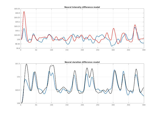
I simulated 2 conditions of 10 (fast) events to create the BOLD time course in two voxels. In one voxel the stimulus duration is 0 (simulating some regions responding to the presentation of the stimulus) but intensities are changing, in the other voxel, intensities are fixed and neural duration are changing.

Figure 1. Simulated BOLD signal in 2 voxels with two conditions. In the intensity approach, the neural intensity changes and we see changes in BOLD signal amplitude as expected. In the duration approach, the neural duration changes, and we see overall changes in shape of the BOLD signal (amplitude and duration).

Then I compare different models in terms of R2 (data fit) and T value (ability to detect the difference). In addition, I looked at how basis functions can inform us on differences in neural durations - the whole code can be found here -

- model 1: GLM with FIR convolved by the hfr only
- model 2: GLM with RT convolved by the hfr only (= variable epoch model)
- model 3: GLM with FIR + PM regressors convolved by the hfr only (= variable impulse model)
- model 4: GLM with FIR + PM regressors convolved by basis functions
- model 5: GLM with mean RT + PM regressors convolved by the hfr only
- model 6: GLM with mean RT + PM regressors convolved by basis functions

Importantly, in models 5 and 6, the mean across all trials and both conditions is used (Munford, 2014). As already showed by Munford (2014), the variable epoch model (nb 3) has reduced power when activation doesn’t scale with RT (i.e. doesn't fit voxel 1).

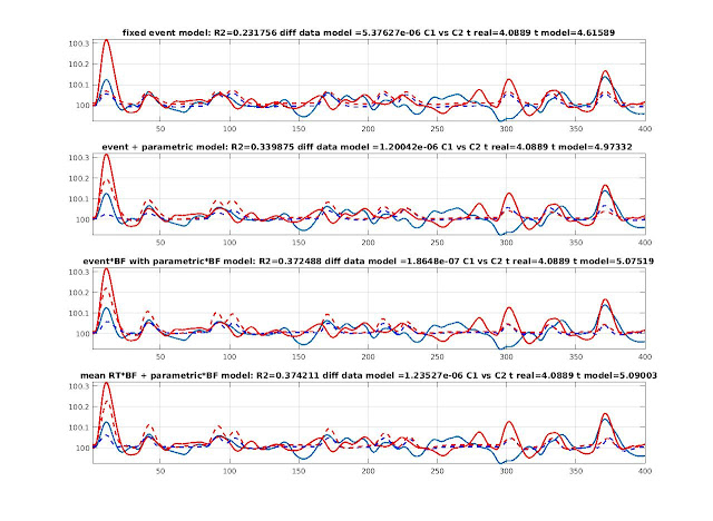
For the voxel where we have neural intensity change, the best models were model 4 and 6 for which we have intensity variations explained by the parametric regressors. Adding BF helped fitting the data since it was a fast event design. The epoch model (mode 2) was the poorer. Using mean RT + parametric did not do a good job because of the time delay introduced by the mean RT. The last model (model 6) clearly outperform model 3. For simplicity I show below models 3, 4 and 6 (figure 2). Importantly in model 6, the time derivative is what allowed the mean RT regressor to fit well the data.

Figure 2. BOLD signal (blue and red) produced by variable neural intensities fitted with event and parametric regressors convolved by the hrf (model 3 - top) or the hrf and derivatives (model 4 - middle) and blocks (mean RT = 4 sec) with parametric regressors convolved by the hrf and derivatives (model 6 - bottom). Dashed lines show modeled data.

For the voxel where we have neural duration change, the best model was again model 6: mean RT + parametric with basis functions, it performed just above the variable epoch model (model 2). Without basis function, it stills performed well but just below the fixed event with parametric and BF. The worst models were the fix event, with or without parametric regressors. Only adding basis functions helped. For simplicity I show below models 2, 4 and 6 (figure 3). Importantly in model 6, this was the dispersion derivative that allowed to match variations of amplitudes.

Figure 3. BOLD signal (blue and red) produced by variable neural durations fitted with block regressors (each block = RT) convolved by the hrf (model 2 - top), with event with parametric regressors convolved by the hrf and derivatives (model 4 - middle) and blocks (mean RT = 4 sec) with parametric regressors convolved by the hrf and derivatives (model 6 - bottom). Dashed lines show modeled data.

In conclusion, I would say that a GLM with mean RT + PM regressors convolved by basis functions is the optimal choice, fitting voxels with amplitude changes that reflect either neural intensity or duration changes - for overall conditions effects, the coefficients of BF for the mean RT and for the PM can be pooled as described in Pernet 2014, thus reflecting the data fit. However, it is important to also explore the role of the time and dispersion derivatives on the mean RT regressors. Counter-intuitively, an effect of the time derivatives suggests differences in neural intensities and an effect of  dispersion derivatives suggest differences in neural durations.

The same neural computation is performed with identical time and intensity, but the metabolic expenditure differs between the groups.

The example is that 'the groups could differ in the amount of transmitter release, the nature of neurovascular coupling (e.g. due to differences in contact between astrocytes and neurons), or the degree to which they rely upon oxidative versus non-oxidative metabolism'.

When it comes to compare different group ages, there is nothing to argue - Poldracks argument are clear cut: 'any changes in neuronal structure could potentially result in changes in energy usage; the time course of any such changes appears to be currently unknown. Similarly, changes in the nature of synaptic signaling, such as the well known changes in synaptic density (i.e. “pruning”) that accompany brain development along with changes in the relative abundance of NMDA receptors and metabotropic signaling, could impact the relative efficiency of signaling with development. [...] The brain's use of these different energetic pathways is known to vary with development. In particular, a recent meta-analysis by Goyal et al. (2014) showed that aerobic glycolysis is greatly increased during childhood, and that regional increases in glycolysis are associated with expression of genes related to synaptic development'. In addition to these changes, I also want to point out here the major role played by astrocytes in learning and synapse regulation - in addition to their role in controlling the blood flow. Little is known about how they change during aging and disease but I'd think this can influence the signal as well.

So what it tells us, is that group differences can be related by underlying difference in energy budget. Luckily, resting state fluctuation are also likely to be influenced by these factors (in fact some argue that part of these fluctuations reflect metabolic activity). In addition, we know that during a task these fluctuation are below the evoked responses (slightly sub-additive). Therefore, comparing the resting state activity between 2 groups, can help interpreting the task based BOLD differences.