Assessing anatomical brain parcellation
Rational
Anatomical brain parcellation is used in three scenarios: (1) identify a brain region to measure some level of activity, for instance, changes in BOLD or tracer concentration, (2) determine the anatomical properties of brain regions, for instance, volume or thickness, (3) use parcels to calculate connectivity values, for instance, rsfMRI correlations or the average number of streamlines in DTI. Given these applications, making sure the right regions and borders are obtained is therefore essential. Dr Shadia Mikhael (graduated in Septembre) looked into that under my supervision, and she did well :-)
Where are we? (as in 2019)
Part 1: protocols
In Mikhael et al (2017) we reviewed in details how anatomical parcels were made, that is how borders are defined and on the basis of what atlases/templates. Surprisingly, the main contenders, FreeSurfer, BrainSuite and BrainVISA have some serious issues.
There are little details on the reference population used: sex ratio, ethnicity, age, education, handedness, etc. In general, software relies on small numbers of participants sometimes averaging across ages and ethnicities. Perhaps related to this point, accounting for anatomical variability is not always explicit. The gyral parcels, or gyral volumes, are regions bound by the grey matter, or pial, layer on the exterior, and the WM layer on the interior in all software (+ sulcal derived regions in BrainVisa). The issue, however, is that some regions are defined relative to each other. Practically this means that after landmarks are defined and some regions found, you could find definitions of the medial border of region A defined by region B and then the lateral border of region B defined by region A, so where exactly is the border? and this causes big problems when accounting for anatomical variability such as branching, interruptions and even double gyri.
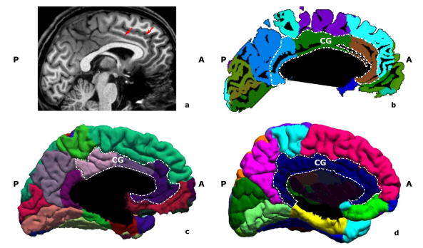
sub-01 from http://psydata.ovgu.de/studyforrest/
despite a clear double cingulate, software packages can fail to capture it all, with a knock-on effect on neighbouring parcels (let's hope such variations are not more frequent in some patient populations or all our analyses are wrong)
Part 2: software assessment
To assess if those differences in protocol matters, we created i) a protocol (for 4 regions) that identifies borders from landmarks only and explicitly accounts for variability; ii) a dataset of manually segmented regions using this protocol iii) a software (Mikhael and Gray, 2018) to compute volume, thickness, surface area from binary images and iv) ran some basic comparisons against FreeSurfer, since some measures were validated against histology (Mikhael et al, 2019).
Some interesting insights came out of this:
- creating a protocol that leads to the unambiguous definition of a region is hard. There are many variations across individuals and being able to define how to always find each border requires multiple cases description.
- manual segmentation is tricky. Even with a detailed protocol, some borders can be inconsistent and inter-rater agreement is still necessary.
- there are so many assumptions to make when deriving morphometric values, and the issue is that those assumptions are, for the most part, not explained in software we use. Take for instance thickness. Should you measure the shortest distance from every voxel and average those, or maybe take the orthogonal projection from one side of the gyrus to the other (and vice versa) and average those? we choose, like FreeSurfer, the second option. Come then the problem of folds, when you have a curve and work with voxels, the orthogonal projection can shoot right between voxels on the other side .. that's ok let's remove this projection. How many projections to compute (step size) and what to remove then? this is just a simple example, but I think not knowing all those decisions in the software can create problems, especially if one wants to compare results from 2 different studies that used different software (even assuming regions match roughly).
Part 3: What to do with variablity?
The final part of this work was to compare outputs from software, using our parcels as a reference frame. Since we know software packages have different borders and so on, we expect differences. This is like saying let's compare the GDP of France using Euros and of the UK using Sterlings - well yeh it's different. Now if we compute each package metric relative to our manually derived values, there are in the same unit, just like comparing GDP on France and UK in US dollars.
In Mikhael and Pernet (2019) we did just that and found: i) as expected from the protocol analysis, that anatomical variablity is not well accounted for; even missing double cingulate gyri! ii) volume and surface areas are mostly affected by this problem since parcel sizes change (while thickness even if from the wrong region, would need dramatic changes to create big differences on average) iii) multiatlas registration is the most accurate.
Violin plots show ROI cortical volume in cm3 computed by Masks2Metrics (M2M), FreeSurfer (FS-DK, FS-DKT), BrainSuite (BS), and BrainGyrusMapping (BGM) (the middle lines represent the medians, boxes the 95% Bayesian confidence intervals, and the density of the random average shifted histograms). Line plots show the relative difference from each package (FS, BS, BGM) to the ground truth estimates (M2M) for each subject (each line is a subject). Double CG occurrences were observed for subjects 1, 5, 6, and 8 in the left hemisphere, and subjects 6 and 10 in the right hemisphere. BrainSuite failed for subjects 4 and 6
Conclusion
For the time being, if you have a good multiatlas tool for parcellating, this is likely to most efficient. The issue is that those, for now, will only give you regions to possibly compute volumes. This means to address goals 1 and 3 listed in the rational, this is my to go to option. If you want to derive morphometrics, then manual editing is required, yes even for those 600 cases you have to process.
References
Data
protocol // MRI data // software // code and resultsArticles
Mikhael et al (2017) Critical Analysis of NeuroAnatomical Software Protocols Reveals Clinically Relevant Differences in Parcellation Schemes. NeuroImage.
Mikhael and Gray. Masks2Metrics (M2M): A Matlab Toolbox for GoldStandard Morphometrics. JOSS
Mikhael et al (2019) Manually-parcellated gyral data accounting for all known anatomical variability. Sci Data
Mikhael and Pernet (2019) A controlled comparison of thickness, volume and surface areas from multiple cortical parcellation packages. BMC Bioinformatics
Mikhael et al (2019) Manually-parcellated gyral data accounting for all known anatomical variability. Sci Data
Mikhael and Pernet (2019) A controlled comparison of thickness, volume and surface areas from multiple cortical parcellation packages. BMC Bioinformatics


Comments
Post a Comment